Party Unity Scores
Jeff Lewis
March 28, 2026
Overview
Here we describe how we create and continue the Party Unity Scores that Keith Poole previously posted here. We produce both member- and Congress-level unity data. We also include a figures showing the change in the scores over time and compare these new scores to the ones previously produced by Poole.
You can download a Congress-chamber party unity summary here and a member level party unity scores here.
Two-party systems
Poole provided party unity scores for all Congresses in which there were two dominant parties. Those are the first through the 17th, the 19th through the 30th and the 35th through the present. Poole describes the two earlier two-party systems on the web page linked above as follows:
The files below are the same as those posted above only now the Jeffersonian-Republican/Federalist (Congresses 1 - 17, 1789 - 1822) and the Democrat/Whig (Congresses 19 - 30, 1825 - 1848) systems are also included in the files. For Congresses 1 - 3 party code 4000 (Anti-Administration) was treated as Jeffersonian-Republican and party code 5000 (Pro-Administration) was treated as Federalist. For Congresses 19 and 20 party code 555 (Jackson) was treated as Democrat and party code 22 (Adams) was treated as Whig. For Congresses 21 - 24 party code 1275 (Anti-Jackson) was treated as Whig (party code 555 also used for Democrat during this period).
Loading and processing the data
We begin by loading the most recent member data from Voteview.com so that we can append parties to the roll call voting data.
member_dat <- read_csv("https://voteview.com/static/data/out/members/HSall_members.csv", col_types = cols())We then identify the major parties in each Congress:
big_party <- member_dat |>
                filter(chamber != "President" &
                       !(congress %in% c(18, 31:34))) |>
                summarize(num=n(), .by=c(congress, chamber, party_code)) |>
                slice_max(num, n=2, by=c(congress, chamber)) |>
                select(-num)
We can then use this dataframe to subset the master data down to just the votes cast by major party members.
major_dat <- read_csv("https://voteview.com/static/data/out/votes/HSall_votes.csv", col_types = cols()) |>
            left_join(member_dat, by = c("congress", "chamber", "icpsr")) |>
        select(congress, chamber, rollnumber, icpsr, bioname, party_code, state_abbrev, district_code, cast_code) |>
            right_join(big_party, by =  c("congress", "chamber", "party_code"))
rm(member_dat)
Party unity votes by Congress
vote_code_map <- c(1,1,1,2,2,2,0,0,0)
unity_votes <- major_dat |>
                  mutate(cast_code = vote_code_map[cast_code]) |>
                  filter(cast_code != 0) |>
                  summarize(n=n(), .by=c(congress, chamber, rollnumber, party_code, cast_code)) |>
                  filter(n()==1 | n>min(n), .by=c(congress, chamber, rollnumber, party_code)) |>
                  summarize(unity = min(cast_code) != max(cast_code),
                            .by=c(congress, chamber, rollnumber))

unity_votes_by_congress <- unity_votes |>
                  summarize(unity_votes = sum(unity),
                            total_votes = n(),
                            .by = c(chamber, congress)) |>
                  mutate(percent_unity = unity_votes/total_votes) |>
                  pivot_longer(cols = c(unity_votes, total_votes, percent_unity),
                               names_to = "fld", values_to = "val") |>
                  unite(chamber_fld, chamber, fld) |>
                  pivot_wider(names_from = chamber_fld, values_from = val) |>
                  rename_with(tolower)
write_csv(unity_votes_by_congress, file="party_unity_by_congress.csv")
head(unity_votes_by_congress)
## # A tibble: 6 × 7
## congress house_unity_votes house_total_votes house_percent_unity
## <dbl> <dbl> <dbl> <dbl>
## 1 1 65 109 0.596
## 2 2 75 102 0.735
## 3 3 55 69 0.797
## 4 4 55 83 0.663
## 5 5 130 155 0.839
## 6 6 82 96 0.854
## # ℹ 3 more variables: senate_unity_votes <dbl>, senate_total_votes <dbl>,
## # senate_percent_unity <dbl>Comparing the new results to Poole’s scores
Now let’s compare what we find using the new data to the scores last reported by Poole. We begin by loading Poole’s party unity scores from the legacy voteview webpage.
poole_unity_by_congress <- read_table("https://legacy.voteview.com/k7ftp/partyunity_house_senate_1-113.dat",
                                       col_names=c("congress", "year", "house_total_votes",
                                                  "house_unity_votes", "house_percent_unity",
                                                  "house_prop_maj_fwr", "house_prop_maj_jd",
                                                  "senate_total_votes", "senate_unity_votes",
                                                  "senate_percent_unity", "senate_prop_maj_fwr",
                                                  "senate_prop_maj_jd"),
                                      col_types = cols(congress = col_integer(),
                                   house_total_votes = col_integer(),
                               house_unity_votes = col_integer(),
                               house_percent_unity = col_double(),
                                                       house_prop_maj_fwr = col_double(),
                               house_prop_maj_jd = col_double(),
                                                       senate_total_votes = col_integer(),
                               senate_unity_votes = col_integer(),
                                                       senate_percent_unity = col_double(),
                               senate_prop_maj_fwr = col_double(),
                                                       senate_prop_maj_jd = col_double()))
## Warning: 10 parsing failures.
## row col expected actual file
## 18 senate_total_votes no trailing characters 0.00000 'https://legacy.voteview.com/k7ftp/partyunity_house_senate_1-113.dat'
## 18 NA 12 columns 9 columns 'https://legacy.voteview.com/k7ftp/partyunity_house_senate_1-113.dat'
## 31 senate_total_votes no trailing characters 0.00000 'https://legacy.voteview.com/k7ftp/partyunity_house_senate_1-113.dat'
## 31 NA 12 columns 9 columns 'https://legacy.voteview.com/k7ftp/partyunity_house_senate_1-113.dat'
## 32 senate_total_votes no trailing characters 0.00000 'https://legacy.voteview.com/k7ftp/partyunity_house_senate_1-113.dat'
## ... .................. ...................... ......... .....................................................................
## See problems(...) for more details.We then stack the old and the new scores.
library(ggplot2)

firstup <- function(x) {
   substr(x, 1, 1) <- toupper(substr(x, 1, 1))
   x
}

glimpse(unity_votes_by_congress)
## Rows: 114
## Columns: 7
## $ congress <dbl> 1, 2, 3, 4, 5, 6, 7, 8, 9, 10, 11, 12, 13, 14, 15…
## $ house_unity_votes <dbl> 65, 75, 55, 55, 130, 82, 112, 95, 90, 140, 208, 2…
## $ house_total_votes <dbl> 109, 102, 69, 83, 155, 96, 142, 132, 158, 237, 29…
## $ house_percent_unity <dbl> 0.5963303, 0.7352941, 0.7971014, 0.6626506, 0.838…
## $ senate_unity_votes <dbl> 52, 25, 57, 66, 146, 90, 61, 86, 47, 54, 90, 126,…
## $ senate_total_votes <dbl> 97, 51, 79, 86, 202, 120, 88, 150, 88, 91, 166, 2…
## $ senate_percent_unity <dbl> 0.5360825, 0.4901961, 0.7215190, 0.7674419, 0.722…## Rows: 113
## Columns: 12
## $ congress <int> 1, 2, 3, 4, 5, 6, 7, 8, 9, 10, 11, 12, 13, 14, 15…
## $ year <dbl> 1789, 1791, 1793, 1795, 1797, 1799, 1801, 1803, 1…
## $ house_total_votes <int> 109, 102, 69, 83, 155, 96, 142, 132, 158, 237, 29…
## $ house_unity_votes <int> 70, 75, 56, 56, 131, 82, 112, 97, 91, 144, 208, 2…
## $ house_percent_unity <dbl> 0.64220, 0.73529, 0.81159, 0.67470, 0.84516, 0.85…
## $ house_prop_maj_fwr <dbl> 0.69734, 0.72631, 0.82763, 0.82283, 0.88838, 0.89…
## $ house_prop_maj_jd <dbl> 0.68955, 0.76163, 0.78050, 0.85626, 0.91968, 0.92…
## $ senate_total_votes <int> 100, 52, 79, 86, 202, 120, 88, 150, 88, 91, 167, …
## $ senate_unity_votes <int> 52, 27, 58, 67, 147, 91, 61, 91, 50, 56, 97, 130,…
## $ senate_percent_unity <dbl> 0.52000, 0.51923, 0.73418, 0.77907, 0.72772, 0.75…
## $ senate_prop_maj_fwr <dbl> 0.66468, 0.68689, 0.84148, 0.84467, 0.84267, 0.86…
## $ senate_prop_maj_jd <dbl> 0.79195, 0.68841, 0.85766, 0.89031, 0.87948, 0.93…ubc <- bind_rows(unity_votes_by_congress |> mutate(version="New"),
poole_unity_by_congress |>
mutate(version="Poole") |>
filter(!(congress %in%c(18,31:34)))) |>
select(contains("percent"), congress, version) |>
pivot_longer(cols = contains("percent"), names_to = "chamber", values_to = "percent") |>
mutate(chamber = firstup(sapply(str_split(chamber, "\\_"), function(x) x[[1]])))Finally, we can make a plot to compare the two sets of unity scores.
ggplot(ubc,
       aes(x=congress*2 + 1787,
           y=percent*100,
           group=version,
           color=version
           )) +
   facet_wrap(~chamber) +
   geom_line(alpha=0.75) +
   ylab("Percent Party Unity Rollcalls") +
   scale_x_continuous("Year", breaks=seq(1790,2022,by=20)) +
   theme_minimal() +
   theme(axis.text.x = element_text(angle = 45, hjust = 1))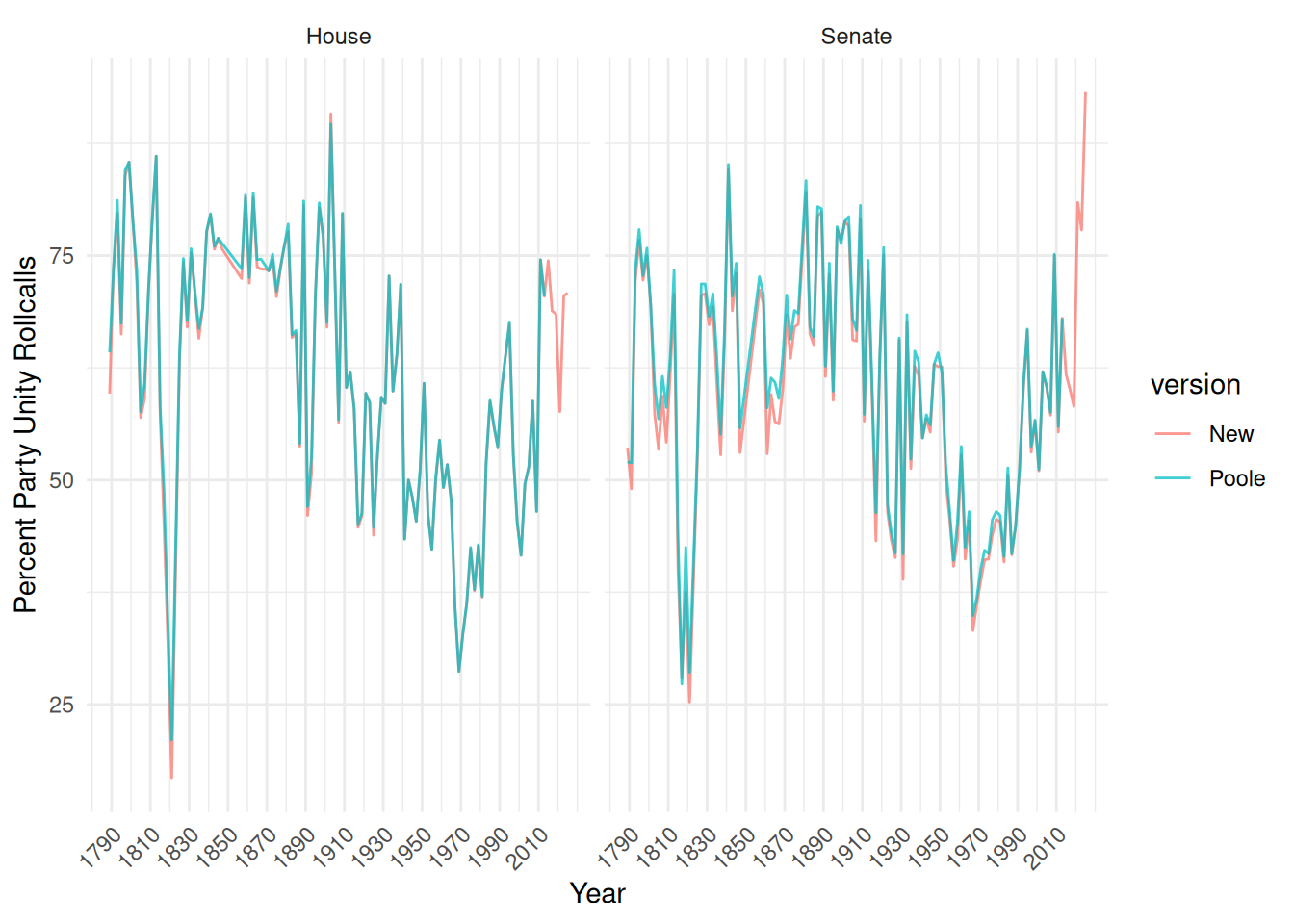
Overall, the two sets of scores line up very closely. The orange line for the new scores is often hidden behind the green line for Poole’s scores. It appears that when the scores differ, the new scores are slightly higher and that the differences are more common in the Senate than in the House. We are not sure what accounts for these differences. We have cleaned up a number of errors in the data in constructed the new Voteview. There could also be differences in the exact criteria used for establishing whether a vote was a unity vote.
Member voting on unity votes
Poole provided data on the rate at which each member voted with their party on party unity votes. We will reproduce and continue those data here.
We limit the votes to just those that are party unity votes as determined above. We filter out the voters from prior to the 35th Congress as well as all of the abstentions and missed votes.For every congress, chamber, roll call and party, we determine the modal vote. We then count the number of times that each member voted with the modal member of their party across party unity votes.
party_unity_members <- major_dat |>
          right_join(unity_votes |> filter(unity),
                    by = c("congress", "chamber", "rollnumber")) |>
          filter(congress > 34) |>
          mutate(cast_code = vote_code_map[cast_code]) |>
          filter(cast_code > 0) |>
          mutate(party_maj_choice = median(cast_code), .by = c(congress, chamber, rollnumber, party_code)) |>
          summarize(total_unity_votes=n(),
                    with_party_unity_votes = sum(cast_code==party_maj_choice),
                    .by = c(congress, chamber, icpsr, bioname, party_code, state_abbrev, district_code)) |>
          mutate(party_unity_score = with_party_unity_votes/total_unity_votes )

write_csv(party_unity_members, file="party_unity_by_member.csv")
rm(major_dat)
Comparing to Poole’s estimates
flds <- fwf_widths(c(4, 6, 3, 2, 8, 5, 12, 8, 7, 7),
                   c("congress", "icpsr", "state_code",
                     "cd", "state", "party_code",
                     "name", "party_unity_score",
                     "with_party_unity_votes",
                     "total_unity_votes"))

ctypes <- cols(
  congress = col_integer(),
  icpsr = col_integer(),
  state_code = col_character(),
  cd = col_character(),
  state = col_character(),
  party_code = col_character(),
  name = col_character(),
  party_unity_score = col_double(),
  with_party_unity_votes = col_integer(),
  total_unity_votes = col_integer()
)

poole_party_unity_members  <- bind_rows( read_fwf("https://legacy.voteview.com/k7ftp/Senate_Party_Unity_35-113.DAT",
                                                     col_positions=flds,
                                                     col_types=ctypes) |>
                                           mutate(chamber="Senate"),
                                         read_fwf("https://legacy.voteview.com/k7ftp/House_Party_Unity_35-113.DAT",
                                                    col_positions=flds,
                                                    col_types=ctypes) |>
                                           mutate(chamber="House") )
Now, we merge new and old scores and compare in a plot.
tg <- left_join(poole_party_unity_members, party_unity_members,
          by=c("icpsr", "chamber", "congress"))

ggplot(tg, aes(x=party_unity_score.x,
               y=party_unity_score.y*100,
               size=total_unity_votes.x)) +
       geom_point(alpha=0.1) +
       theme_minimal() +
       geom_abline(intercept=0, slope=1, col='red') +
       coord_equal() +
       xlab("New party unity scores") +
       ylab("Poole party unity scores") +
       theme(legend.title=element_blank())
## Warning: Removed 612 rows containing missing values or values outside the scale range
## (`geom_point()`).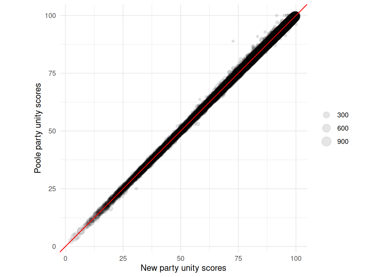
Most of the scores are very similar across the two datasets.